1 Transforming a density

Suppose we have

a real-valued random variable $X$ with density $f$ (with respect to the standard measure on the real line), and
another random variable $Y$ which is defined as a deterministic function $X$, denoted $y(x)$.

Assume that $y$ is a monotonic invertible function, so the inverse function $x(y)$ is also well-defined.Let’s also assume it is monotonically increasing for now. We’ll see we can drop that assumption later, and allow monotonically decreasing functions too.

Question: what is the pdf of $Y$?

First note: by definition, $\Pr(a\le X\le b) = \int_a^b f(x)\dee{x}$.

Given our assumptions about the function $y$, we have that $a\le X\le b\implies y(a)\le Y\le y(b)$.

So, using differentiation by substitutionRecall, this follows simply from the chain rule, where the CDF $F$ is the antiderivative of $f$: \[ \begin{aligned} &\phantom{=}\int_{y(a)}^{y(b)}f(x(y))\frac{\dee}{\dee{y}}x(y)\dee{y}\\ &=\int_{y(a)}^{y(b)}\frac{\dee}{\dee{y}}F(x(y))\dee{y}\\ &=F(x(y(b)))-F(x(y(a)))\\ &=F(b)-F(a)\\ &=\int_{a}^{b}f(x)\dee{x} \end{aligned} \]

\[ \begin{aligned} \Pr(y(a)\le Y\le y(b)) &= \Pr(a\le X\le b) \\ &= \int_a^b f(x) \dee{x}\\ &= \int_{y(a)}^{y(b)} f(x(y)) \frac{\dee{x(y)}}{\dee{y}}\dee{y} \end{aligned} \]

So the pdf of $Y$ is $f(x(y)) \frac{\dee{x}(y)}{\dee{y}}$.

If $y$ is monotonically decreasing, then we have to switch the limits on the integral, but we also get a negative sign in the derivative (see this math.SE answer). Thus, we can say in general

\[\text{The pdf of $Y$ is }g(y) \coloneqq f(x(y)) \left|\frac{\dee{x}(y)}{\dee{y}}\right|\]

The above explanation can be found in multiple sources, but for me to get a better understanding, it helped to look at some examples, and plot them. A key insight here can be gotten by thinking about what happens to some interval in the domain of $f$. Integrating the density $f$ over this interval will give the same result as integrating the transformed density $g$ over whatever the image of the interval is, under the transformation.

This intuition is helpful to play with when relating this perspective on random variables to a measure theoretic one that uses the concept of pushforwards.

2 Examples

Some examples with pictures helped me understand what this means. Here’s a first example:

let $X$ be a random variable with density $f(x) = \frac2\pi\sqrt{1-x^2}$ (restricted to $-1 \le x \le 1$).
and let $Y$ be the random variable defined by $y(x) = \arcsin x$, which is monotonically increasing.

Then $x = \sin y$ and $\frac{\dee x(y)}{\dee y} = \cos y$, so the density of $Y$ is

\[g(y) = f(x(y))\frac{\dee x(y)}{\dee y} = \frac2\pi\sqrt{1-\sin^2}\cos y = \frac2\pi\cos^2y\]

Show/hide code

using Plots

function plot_transform_pdf(;
        f, y, g,
        xlim,
        demo_range = (0.4, 0.7),
        resolution = 100, size = (500,500),
        plotlims=nothing)
    (xmin, xmax) = xlim
    dx = (xmax-xmin)/resolution
    xs = xmin:dx:xmax
    xmin_ = xmin+demo_range[1]*resolution*dx
    xmax_ = xmin+demo_range[2]*resolution*dx
    xs_ = xmin_:dx:xmax_
    if plotlims!==nothing
        xlim=plotlims
    else
        xlim=(min(minimum(xs),
                  minimum(y.(xs)),
                  minimum(f.(xs)),
                  minimum(g.(y.(xs)))),
              max(maximum(xs),
                  maximum(y.(xs)),
                  maximum(f.(xs)),
                  maximum(g.(y.(xs)))),)
        if any(isinf.(xlim))
            @warn """
            plotlims=$(xlim) contains nonfinite value(s).
            Plot may not display correctly.
            To set manually, use `plot_transform_pdf(... , plotlims=(min, max))`.
            """
        end
    end
    ylim=xlim

    ys = y.(xs)
    ys_ = y.(xs_)

    l = @layout [[f _]; [y g]]

    pf = plot(xs, f.(xs), xaxis=false, xticks = false,
        label = "f(x)", color = :red,
        ylabel="f(x)",
        xlim=xlim, ylim=ylim)
    pg = plot(g.(ys), ys, xlabel="g(y)",
        label = "g(y)", color = :blue,
        yaxis = false, yticks = false,
        xlim=ylim, ylim=xlim) #note swapped axes
    px = plot(xs, y.(xs), xlabel="x", ylabel="y", color = :gray,
        label = nothing,
        xlim=xlim, ylim=ylim)
    plot!(pf,
        [xs_'; xs_'], [fill(0.0, length(xs_))' ; (f.(xs_))'],
        lc=:green, label=false, alpha = 0.5)
    plot!(pg,
        [fill(0.0, length(ys_))' ; (g.(ys_))'], [ys_'; ys_'],
        lc=:green, label=false, alpha = 0.25)
    scatter!(px, xs_, y.(xs_),
        color=:green, label = false, markersize=2, msw=0, alpha = 0.25)
    plot!(px,
        [xs_' ; fill(xlim[2], length(xs_))'], [ys_'; ys_'],
        lc=:gray, label=false, alpha = 0.1)
    plot!(px,
        [xs_' ; xs_'], [ys_'; fill(xlim[2], length(ys_))'],
        lc=:gray, label=false, alpha = 0.1)
    plot(pf, px, pg, layout = l, size = size, fmt=:svg)
end;

Show/hide code

plot_transform_pdf(
    f = x -> 2/pi * sqrt(1-x^2),
    y = x -> asin(x),
    g = y -> 2/pi * cos(y)^2,
    xlim = (-1, 1),
    demo_range = (0.7, 0.9), resolution = 100
)

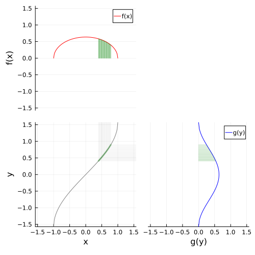
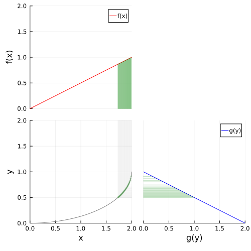
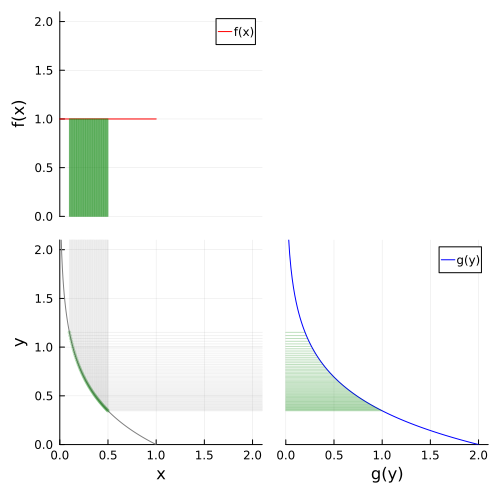
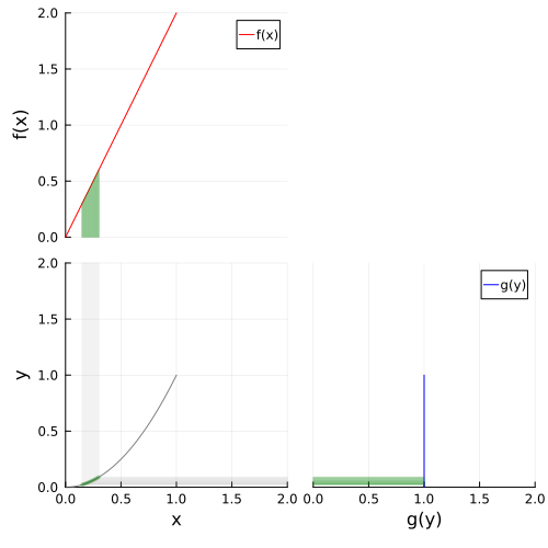
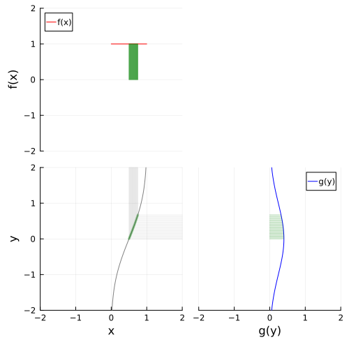
Figure 1: A semicircle density transformed by y(x)=\arcsin x. — Figure 1: A semicircle density transformed by $y(x)=\arcsin x$.

Legend

upper left: ${\color{red}f(x)}$, the pdf of $X$
lower left: the invertible mapping between $x$ and $y$
lower right: ${\color{blue}g(y)}$, the pdf of $Y$ (plotted with $y$ on the vertical axis and density $g(y)$ on the horizontal axis, so the axes line up).

The green lines shade an example area under the curve to show how probability of an event is preserved (area is preserved under this transform), and how this region is transformed between $x$ and $y$.

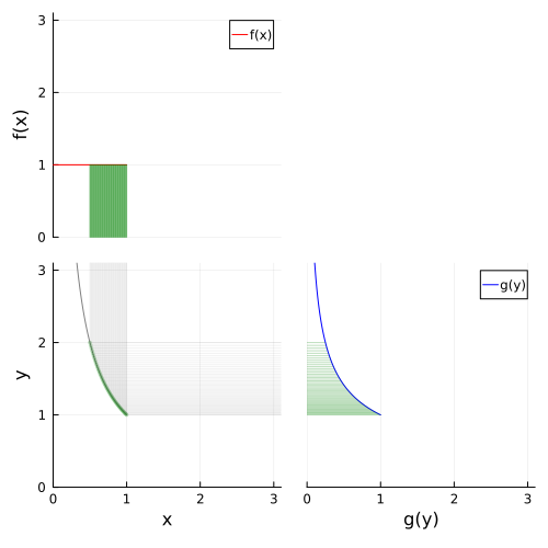
Here is another example, transforming uniform to Pareto distribution:

let $X\sim\mathrm{Uniform}(0,1)$, so pdf $f(x)=1$
let $Y$ be defined as $y(x) = x^{-1}$, which is monotonically decreasing over the range $y>0$.

Then $x = y^{-1}$ and $\frac{\dee x(y)}{\dee y} = -{y^{-2}}$, so the density of $Y$ is

\[g(y) = f(x(y))\left|\frac{\dee x(y)}{\dee y}\right| = {y^{-2}}\]

Thus $Y\sim\mathrm{Pareto}(1,1)$The pdf of a $\mathrm{Pareto}(\kappa,\alpha)$ is \[\mathrm{pdf}(z)=\alpha\kappa^\alpha z^{-(\alpha+1)}\] over range $z\ge\kappa$

Show/hide code

plot_transform_pdf(
    f = x -> 1,
    y = x -> 1/x,
    g = y -> 1/y^2,
    xlim = (0, 1),
    plotlims = (0, 3.1), # set manually, since goes to infinity
    demo_range = (0.5, 1.0), resolution = 100
)

Figure 2: A uniform density transformed by y(x)=x^{-1}, giving a Pareto distribution. — Figure 2: A uniform density transformed by $y(x)=x^{-1}$, giving a Pareto distribution.

More examples

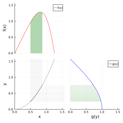
The following are some more examples (taken from here).

- let $X$ have pdf $f(x) = 2 x \cos{x^2}$ for $0\le x \le \sqrt{\pi/2}$ (and $0$ elsewhere)
- let $Y$ be defined as $y(x) = x^2$, which is monotonically increasing in the range.
Then $x=\sqrt{y}$, and $\frac{\dee x(y)}{\dee y} = \frac1{2\sqrt{y}}$, so the density of $Y$ is

\[g(y) = f(x(y))\frac{\dee x(y)}{\dee y} = 2 \sqrt y \cos y\frac1{2\sqrt y} = \cos y\]

Show/hide code

plot_transform_pdf(
    f = x -> 2x * cos(x^2),
    y = x -> x^2,
    g = y -> cos(y),
    xlim = (0, √(π/2))
)

Figure 3: Example 1: the squaring map y(x)=x^2 gives a cosine density. — Figure 3: Example 1: the squaring map $y(x)=x^2$ gives a cosine density.

- let $X$ have pdf $f(x) = x/2$ for $0\le x \le 2$ (and $0$ elsewhere)
- let $Y$ be defined as $y(x) = 1-\sqrt{4-x^2}/2$ (again, monotonically increasing).
Then $x=2\sqrt{y(2-y)}$, and $\frac{\dee x(y)}{\dee y} = \frac{2(1-y)}{\sqrt{y(2-y)}}$, so the density of $Y$ is

\[g(y) = f(x(y))\frac{\dee x(y)}{\dee y} = \frac{2\sqrt{y(2-y)}}{2}\frac{2(1-y)}{\sqrt{y(2-y)}}=2(1-y)\]

Show/hide code

plot_transform_pdf(
    f = x -> x/2,
    y = x -> 1-√(4-x^2)/2,
    g = y -> 2(1-y),
    xlim = (0, 2),
    demo_range = (√3/2, 1), # a range that gives 1/4 of total area
    resolution = 200 # let's up the resolution (see denser lines in visualization)
    )

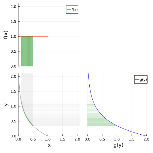
Figure 4: Example 2: a linear density transformed into a triangular one. The demo interval here covers a quarter of the total area.

Transforming a Uniform distribution to an Exponential distribution

let $X\sim \operatorname{Uniform}(0,1)$
let $Y$ be defined as $y(x) = -\frac1\lambda\log(x)$, for some $\lambda > 0$. This is monotonically decreasing.

Then $x=e^{-\lambda y}$, and $\frac{\dee x(y)}{\dee y} = -\lambda e^{-\lambda y}$, so the density of $Y$ is

\[g(y) = f(x(y))\left|\frac{\dee x(y)}{\dee y}\right|= \lambda e^{-\lambda y}\]

So, $Y\sim\operatorname{Exponential}(\lambda)$.

Show/hide code

λ = 2 # set the scale parameter to 2, arbitrarily
plot_transform_pdf(
    f = x -> 1,
    y = x -> -log(x)/λ,
    g = y -> λ*exp(-λ*y),
    xlim = (0, 1),
    plotlims = (0, 2.1), # set manually, since goes to infinity
    demo_range = (0.1, 0.5), resolution=150
    )

Figure 5: Example 3: a uniform density transformed into an exponential one, with \lambda=2. — Figure 5: Example 3: a uniform density transformed into an exponential one, with $\lambda=2$.

Transforming into a Uniform distribution

let $X$ be a random variable with pdf $f(x) = 2x$ for $0\le x \le 1$, and $0$ otherwise.
let $Y$ be defined as $y(x) = x^2$, as in example 1 above, so $x=\sqrt{y}$, and $\frac{\dee x(y)}{\dee y} = \frac1{2\sqrt{y}}$.

Then the density of $Y$ is

\[g(y) = f(x(y)) \frac{\dee x(y)}{\dee y} = 1\]

So, $Y\sim\operatorname{Uniform}(0,1)$. [Verify that the range of $y$ is $[y(0),y(1)]= [0,1]$).]

Show/hide code

plot_transform_pdf(
    f = x -> 2x,
    y = x -> x^2,
    g = y -> 1,
    xlim = (0, 1),
    demo_range = (0.15, 0.3)
)

Figure 6: Example 4: a linear density transformed into a uniform one.

Transforming a Uniform distribution into a Normal distribution

let $X\sim \operatorname{Uniform}(0,1)$, which has pdf $f(x)=1$ for $0\le x \le 1$ and $0$ elsewhere.
let $Y\sim \operatorname{Normal}(0,1)$, which has pdf $g(y) = \frac{1}{\sqrt{2\pi}}e^{-\frac12y^2}$

In this case, we know $g(y)$, but we want to find a function $y(x)$ that will transform $X$ into $Y$. This means we need to solve the differential equation (since $f(x(y)) = 1$):

\[\frac{\dee x}{\dee y} = \frac{1}{\sqrt{2\pi}}e^{-\frac12y^2}\]

This is intractable analytically, but what we need is Y’s inverse CDF. We can use y(x) = quantile(Normal(0,1), x) from Distributions.jl.

Show/hide code

using Distributions
plot_transform_pdf(
    f = x -> 1,
    y = x -> quantile(Normal(0,1), x),
    g = y -> exp(-y^2/2)/sqrt(2π),# = pdf(Normal(0,1),y),
    xlim = (0, 1),
    plotlims=(-2, 2),
    demo_range=(0.5, 0.75)# 1/4 of the total area
)

Figure 7: Example 5: the inverse normal CDF transforms a uniform density into a standard normal one.

We can also revisit example 3 above, and write it the same way (though we need the inverse CDF of 1-x… it’s equivalent.)

Show/hide code

X = Uniform(0, 1)
Y = Exponential(1/2)
plot_transform_pdf(
    f = x -> pdf(X, x),
    y = x -> quantile(Y, 1-x),
    g = y -> pdf(Y, y),
    xlim = (0, 1),
    plotlims = (0,2.1), # set manually, since goes to infinity
    demo_range = (0.1, 0.5)
)

Figure 8: Example 3 again, written with the inverse CDF of the exponential distribution.